Why Transformer Performance Is Mostly a Matmul Problem

Series The Life of a Token Across the LLM Stack 2 / 5

By Wenbo Ji 02 June 2026 17 min read

Two glowing matrix grids flowing through reusable tiles, layered memory bands, compute blocks, and a tiled output grid. Figure 1. Transformer linear algebra as tiled data movement through memory hierarchy and compute blocks. Generated with GPT Image 2.

How Transformer computation maps onto GPU matrix multiplication kernels.

Most expensive operations in a dense Transformer reduce to matrix multiplication. Query, key, and value projections are matmuls. MLP projections are matmuls. The vocabulary projection is a matmul. Once the model has defined those shapes, performance depends on how the GPU moves tiles through memory, feeds tensor cores, and overlaps data movement with computation.

The Transformer view tells us what computation is required. The kernel view tells us whether the hardware can run it efficiently.

This distinction matters because the clean equations in a model diagram are not what the GPU directly executes. A line like Q = XWq hides a lot. It hides how data is loaded from memory, how work is split across thread blocks and warps, how tiles are reused, how tensor cores are fed, and how partial results are accumulated.

Transformer architecture defines the computation graph. Matmul kernels determine how efficiently that graph runs on GPU.

Performance discussions about LLMs keep returning to matrix multiplication for a concrete reason. It is not the only operation in inference, and attention kernels have their own specialized structure. But dense Transformers spend a large share of their FLOPs in matmuls, especially in linear projections and MLPs.

The phrase "mostly a matmul problem" should not be read as "only matmul matters." Layer normalization, elementwise activations, attention score computation, softmax, sampling, communication, and memory allocation all matter. The claim is narrower: if you want to understand where dense Transformer arithmetic goes, you have to understand matrix multiplication. If you want to understand why theoretical FLOPs do not become real throughput, you have to understand how that matrix multiplication moves data.

1. Transformer Computation Becomes Matrix Multiplication

Start with the equations from the previous post:

Q = XW_q,\qquad K = XW_k,\qquad V = XW_v

Here X is the input hidden state for a batch of tokens, and the W matrices are learned projections. The model uses these projections to produce attention queries, keys, and values.

The MLP is also built from linear projections:

\mathrm{MLP}(X) = W_2\left(\sigma(W_0X) \odot W_1X\right)

Depending on notation, the matrices may appear on the left or right, but the core operation is the same: multiply an activation matrix by a weight matrix, optionally apply an elementwise operation, then multiply again.

The final vocabulary projection is another matmul:

\mathrm{logits} = HW_{\mathrm{vocab}}

For a large vocabulary, this can be a meaningful cost, especially when the batch of active decode tokens is small.

In rough form:

The Transformer is a stack of routing operations and feature transformations. The expensive feature transformations are mostly matrix multiplications.

The shapes come from the model and the request. If the active tokens in a batch form an activation matrix with shape M x K, and a projection weight has shape K x N, the output has shape M x N. In prefill, M can be large because many prompt tokens are processed together. In decode, M may be closer to the number of active requests, because each request often contributes one new token. The same weight matrix can therefore be multiplied against very different activation shapes depending on the phase.

In kernel terms, the core projection is:

C_{M \times N} = A_{M \times K} B_{K \times N}

This shape change is one reason inference is harder to reason about than a single benchmark. A large prefill matmul may have enough work to keep tensor cores busy. A small decode matmul may have less parallelism and may spend more relative time on memory movement, kernel launch overhead, or cache reads. The model equation is the same. The hardware problem is not.

Weights are reused across many tokens, while activations are request-specific. A server running one model keeps the same weight matrices resident, but each batch brings new activations, new sequence lengths, and new cache reads. Kernel efficiency depends on how much reuse the current shape allows.

The shape difference is easiest to see in the prefill/decode split. During prefill, a prompt with thousands of tokens can create an activation matrix with many rows. Multiplying that matrix by a projection weight gives the GPU a large amount of regular work. During decode, the active matrix may have one row per running request. If only a small number of requests are active, the operation can become skinny. A skinny matmul can be correct and still be inefficient for the hardware.

2. GPUs Are Built Around Massive Parallelism

Matrix multiplication is a good fit for GPUs because it contains a lot of independent arithmetic. Each output element is a dot product. A large output matrix contains many dot products. Those dot products can be split across many parallel workers.

An NVIDIA GPU is organized around streaming multiprocessors, or SMs. Each SM executes groups of threads called warps. The programmer describes a kernel as many thread blocks; the GPU schedules those blocks across SMs. Modern data-center GPUs also include tensor cores, specialized units designed to accelerate matrix multiply-accumulate operations for formats like fp16, bf16, fp8, and related tensor formats.

At a high level, a GPU does two jobs:

Move and store data.
Do arithmetic on that data.

The second job is what appears in model equations. The first job is what often determines performance.

3. Memory Hierarchy Is the Real Bottleneck

Fast GPU programming is about putting data in the right place at the right time.

Global memory has large capacity but relatively high latency. L2 cache is closer. L1 and shared memory are closer still. Registers are closest to the executing threads. Tensor cores can perform enormous amounts of arithmetic, but they cannot multiply data that has not arrived.

Naive matmul is slow because every output element repeatedly reads the same input values from global memory. The arithmetic may be simple, but the data movement is terrible.

Counting operations is not enough. We also need to ask how many operations we get per byte moved. This is the intuition behind arithmetic intensity. A computation with high reuse can do many multiply-accumulate operations after loading a tile. A computation with poor reuse may spend most of its time waiting for data. GPUs are very good at arithmetic, but they are not exempt from the cost of moving bytes.

The same FLOP count can behave differently across shapes. A matmul with generous dimensions can reuse tiles well. A thin or irregular matmul may expose memory and scheduling overhead. Attention during decode can be especially sensitive because it repeatedly reads KV cache for active sequences. The bottleneck is not always the part that looks largest in a clean equation.

Weight-only quantization is another example of the compute/memory tradeoff. Smaller weights can reduce bandwidth pressure and improve cache residency, but the benefit depends on kernels that can use the compressed format efficiently. If dequantization overhead or unsupported shapes dominate, the expected speedup may not appear. The model-level idea is simple: use fewer bits. The kernel-level result depends on the data path.

High-performance matmul is less about individual multiply-adds than about moving data through the memory hierarchy efficiently.

Reuse is the reason to stage data. If a tile of matrix A and a tile of matrix B are loaded from global memory, the kernel wants to spend that load across many multiply-accumulate operations before discarding the tile. The closer that reuse happens to the compute units, the better.

4. Tiling Is the Central Idea

Tiling turns a huge matmul into many small reusable local computations.

Suppose we want:

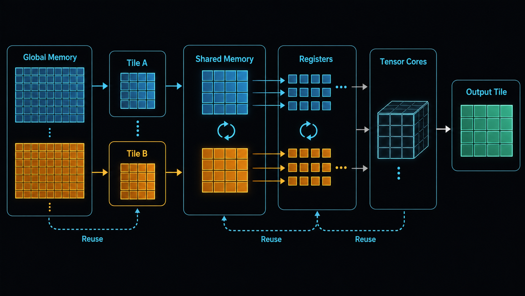
C = A x B

Instead of computing each element independently from global memory, the kernel divides A, B, and C into tiles. A block of threads loads a tile of A and a tile of B into shared memory. Threads then multiply smaller fragments and accumulate partial results in registers. The kernel advances along the reduction dimension, loading the next tiles and accumulating until the output tile is complete.

A small example makes the reuse visible. Imagine one tile of A and one tile of B are loaded from global memory. If those values are used once, the load was expensive. If the same tile values contribute to many output elements before being evicted, the load becomes worthwhile. Shared memory and registers are more than faster storage; they are places where reuse is made explicit.

The picture is:

(A_{\mathrm{tile}}, B_{\mathrm{tile}}) \rightarrow \mathrm{shared\ memory} \rightarrow \mathrm{register\ fragments} \rightarrow \mathrm{tensor\ core\ MMA} \rightarrow C_{\mathrm{tile}}

A diagram of tiled matmul reuse from global memory through shared memory, registers, tensor cores, and output tile. — Figure 2. Tiling makes reuse explicit: global-memory tiles are staged closer to compute so each loaded value contributes to many output elements.

Tiling is an implementation detail with architectural consequences. It is the reason the same value loaded from memory can contribute to many arithmetic operations. That reuse is what makes high throughput possible.

There are many tile levels: thread-block tiles, warp tiles, instruction-level fragments, and tensor-core fragments. Choosing these sizes is a tradeoff among occupancy, register pressure, shared-memory capacity, memory coalescing, and the shape of the matrices.

Those tradeoffs are real. Larger tiles can improve reuse, but they consume more shared memory and registers. More register use can reduce occupancy or cause spilling. Better occupancy can hide latency, but only if the kernel still feeds tensor cores efficiently. Strong kernels are tuned around hardware limits and workload shape, not simply around larger tiles.

For LLM inference, matrix shapes vary by phase. Prefill may involve larger sequence dimensions. Decode may involve small batches of new tokens, where weight loading and KV-cache reads become more visible. The same model equations can stress kernels differently depending on request mix.

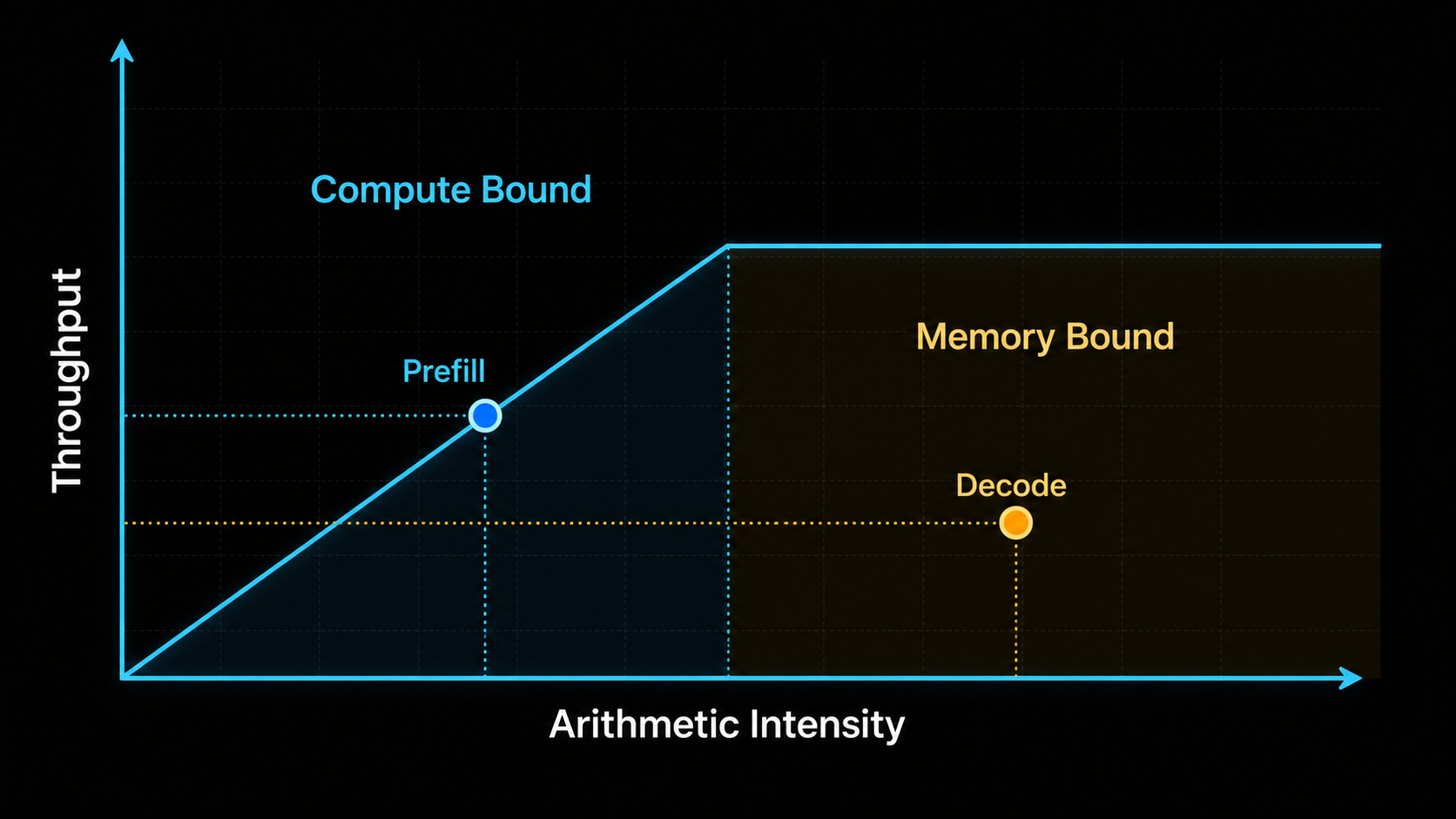
A useful back-of-the-envelope performance model compares arithmetic work to data movement:

T_{\mathrm{op}} \approx \max\left( \frac{\mathrm{FLOPs}}{\mathrm{peak\ FLOP/s}}, \frac{\mathrm{Bytes}}{\mathrm{memory\ bandwidth}} \right)

Arithmetic intensity makes the same point as a ratio:

\mathrm{AI} = \frac{\mathrm{FLOPs}}{\mathrm{Bytes\ moved}}

A roofline-style diagram contrasting prefill and decode across arithmetic intensity, throughput, compute bound, and memory bound regions. — Figure 3. Prefill often gives the GPU more regular matrix work, while decode can move closer to memory-bound behavior because batches are smaller and KV-cache reads matter more.

5. Tensor Cores Change the Unit of Computation

Tensor cores are specialized matrix engines. Instead of thinking only in scalar multiply-add instructions, modern kernels feed tensor cores small matrix fragments. On newer NVIDIA architectures, Hopper/H100 is one example, high-performance kernels may use architecture-specific matrix instructions and asynchronous data movement features to keep the pipeline full.

For NVIDIA GPUs, the programming stack has multiple layers. CUDA is the familiar high-level interface. PTX is a lower-level virtual instruction set. SASS is the actual machine-level instruction form. You do not need to write SASS to understand LLM inference, but the distinction explains why high-performance kernels are architecture-aware. The same mathematical matmul can map to different instruction sequences depending on GPU generation and compiler behavior.

Tensor cores are a capability, not an automatic outcome. The kernel has to present data in a layout and precision the hardware can use. The batch shape has to provide enough independent work. Memory movement has to keep pace. If any of those fail, the operation may use only a fraction of the advertised throughput.

Tensor cores are extremely fast only when the kernel gives them the right work: supported datatypes, compatible layouts, staged fragments, and enough independent matrix work to hide latency.

6. Asynchronous Pipelines Hide Latency

If a kernel loads data, waits, computes, stores, and repeats, it leaves performance on the table. Better kernels overlap these steps.

On architectures with the right support, high-end matmul kernels can move tiles while tensor cores compute on previous tiles. A common pattern is producer-consumer scheduling: some work prepares data movement into shared memory, while other work consumes ready tiles through tensor core operations. Buffers form a small pipeline. As one tile is being used, another tile is being loaded.

The best kernels hide memory latency by overlapping data movement with tensor core execution. If loading, staging, computing, and storing happen as separate blocking phases, expensive compute units sit idle. If the kernel keeps the next tiles in flight while tensor cores consume the current tiles, latency is absorbed into running work.

This pipeline is delicate. Shared-memory layout can create bank conflicts. Register use can become too high and cause spilling. Tile shapes can underuse tensor cores. Memory access patterns can fail to coalesce. Hardware power and clock behavior can also affect sustained throughput.

The model equation hides this pipeline; kernel performance depends on it.

Three implications follow. First, theoretical FLOPs are not delivered token throughput; tensor cores only help when kernels feed them efficiently. Second, inference has shape problems: online traffic mixes prefill and decode, long and short prompts, changing batch sizes, and changing active-request counts. Third, kernel performance depends on serving decisions. Chunked prefill, continuous batching, and paged attention all change the shapes and memory paths that kernels actually see.

The kernel view does not replace the model view or the serving view. It explains the hardware consequences of both.

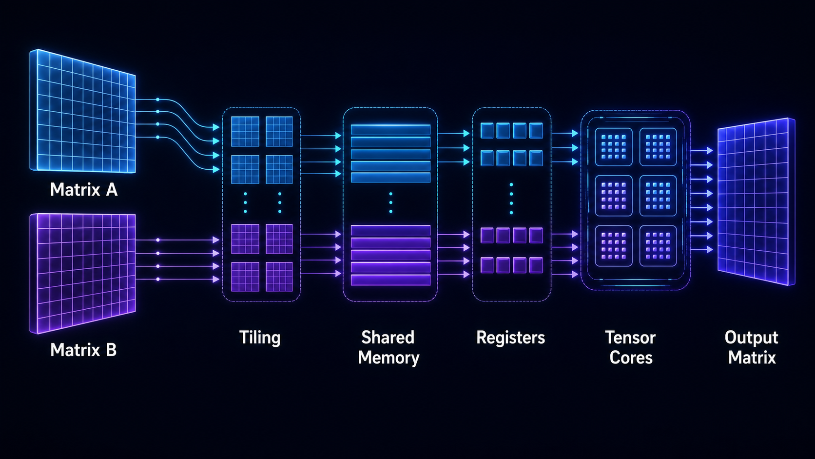
Diagram: Matmul Through the GPU Memory Hierarchy

flowchart LR A["Transformer linear layer"] --> B["Large matrix multiply"] B --> C["Tile A and tile B"] C --> D["Global memory"] D --> E["L2 / L1 cache"] E --> F["Shared memory"] F --> G["Registers"] G --> H["Tensor cores"] H --> I["Output tile"]

The arrows should be read as a data path, not a strict one-time sequence. High-performance kernels pipeline this movement so load, compute, and store overlap.

A Performance Lens for Transformer Operations

When a Transformer operation is slow, ask:

Is the operation large enough to use the GPU well?

Small decode batches may underuse compute because there is not enough parallel work. Large prefill batches may use compute better but consume more memory and delay other requests.

Is the bottleneck arithmetic or memory movement?

MLP matmuls can be compute-heavy. Attention during decode may spend much of its time reading KV cache. The final vocabulary projection can become significant with small batches and large vocabularies.

Are data layouts and precision aligned with hardware?

Tensor cores are optimized for particular fragment shapes and data types. A model using bf16, fp16, fp8, or quantized weights will depend on kernels that exploit those formats correctly.

Does the serving layer produce efficient shapes?

The scheduler can help or hurt. It decides how much work enters a kernel call and how prefill and decode are interleaved.

Here the kernel view meets the serving view. A scheduler that forms larger batches may improve kernel utilization, but larger batches can increase waiting time. Chunked prefill can make long prompts less disruptive, but it also changes the sequence of kernel shapes. Continuous batching can keep decode work flowing, but the active batch may still be too small or too irregular for ideal tensor-core use.

A matmul kernel does not know that one row came from a short chat request and another came from a long document summary. It sees shapes, pointers, layouts, and datatypes. The serving engine is the layer that turns irregular user traffic into those shapes.

GPU utilization has to be read against the workload target. High utilization may come from large prefill work that delays streaming tokens. Low utilization may be acceptable for sparse low-latency traffic. The question is whether the system is using the hardware well for the promised TTFT, inter-token latency, throughput, and tail behavior.

The same kernel can look excellent or mediocre depending on the batch it receives, and that batch is made by the serving layer.

Key Takeaways

Dense Transformer cost is dominated by matmuls in projections, MLPs, and often the vocabulary head.
Delivered throughput depends on data movement, tile reuse, and tensor-core-friendly shapes.
Shared memory, registers, and asynchronous pipelines make expensive loads reusable.
Decode and prefill create different kernel shapes and different bottlenecks.
Serving policy can make strong kernels look better or worse by changing the batches they receive.

References

Aleksa Gordic, Inside NVIDIA GPUs: Anatomy of high performance matmul kernels.
Aleksa Gordic, Inside the Transformer: The Life of a Token.
NVIDIA, NVIDIA Hopper Architecture In-Depth.
NVIDIA, CUTLASS Documentation.

Note: This blog was drafted and polished with the assistance of ChatGPT (GPT-5.4 Thinking), based on my reading notes on Aleksa Gordic's Transformer, matmul, and vLLM articles. Illustrations were generated with GPT Image 2.

← Previous
The Life of a Token Inside a Transformer
Next →
The Life of a Request Inside vLLM