The Life of a Token Inside a Transformer

Series The Life of a Token Across the LLM Stack Part 1 · 6 articles

Wenbo Ji 31 May 2026 17 min read

In brief

A Transformer repeatedly turns each token representation into a context-aware state through normalization, attention, residual updates, and MLP transformations. During decoding, KV cache preserves prior attention state so history is read rather than recomputed.

Embeddings create vectors, while attention and MLP blocks repeatedly refine their contextual meaning.
Positional methods modify how attention interprets token order rather than adding semantic knowledge.
KV cache trades memory capacity for faster autoregressive decoding.

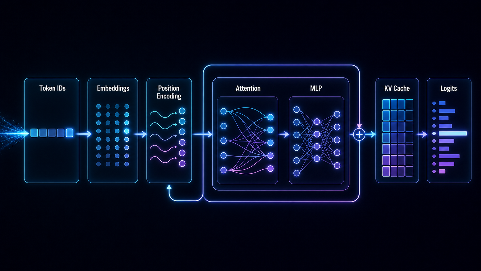
A glowing token vector passing through abstract Transformer blocks with attention arcs, MLP modules, positional waves, KV cache, and logits. Figure 1. A token becoming a contextual hidden state through attention, MLPs, positional structure, and cache state. Generated with GPT Image 2.

How a token becomes a context-aware representation before turning into logits.

Raw language disappears earlier than the API makes it seem. By the time a prompt reaches the model, it is a sequence of token IDs, and then an S x H activation matrix. The Transformer spends the rest of the forward pass changing that matrix, routing information across positions, and producing logits for the next token.

The easiest way to misread a language model is to imagine that it reads text the way we do. The model instead receives token IDs, uses them to select rows from an embedding table, and operates on the resulting sequence of vectors. From that point forward, the Transformer repeatedly transforms and mixes those vectors until it produces logits for the next token.

That mechanical description is the right starting point for inference. Latency, cache size, and GPU work all follow from this vector path.

The core pattern is simple:

MLP changes what a token contains. Attention changes what a token can see.

A Transformer block alternates between these two kinds of work. The MLP is local to each position. It updates the representation of a token without directly looking at other positions. Attention is the communication layer. It lets a token gather information from other allowed tokens in the sequence.

That is the model-level starting point for LLM inference: each generated token is a vector update, an information-routing step, and then a new piece of request state.

1. Text Becomes Tokens, Tokens Become Vectors

The first boundary is tokenization. A tokenizer maps text into a sequence of integer IDs. The model's vocabulary is finite, so arbitrary text has to be represented as pieces from that vocabulary: whole words, word fragments, punctuation, bytes, special control tokens, or other learned units depending on the tokenizer.

Tokenization defines the discrete interface to the model. Once a prompt enters the model, it is no longer one continuous string. It is a sequence:

\mathrm{text} \rightarrow \mathrm{token\ IDs}\ x_{1:S} \rightarrow X = E[x_{1:S}] \in \mathbb{R}^{S \times H}

Each token ID indexes an embedding table. If the hidden size is 4096, each token becomes a 4096-dimensional vector. The exact number depends on the model, but the principle is the same: the integer is only a handle. The vector is what the Transformer operates on.

Special tokens add structure the raw text would not naturally contain: turns, tool calls, fill-in-the-middle regions, end-of-generation events, and other control markers. The tokenizer and prompt formatter shape the computational object that enters the model before the first layer runs.

Once the token embeddings exist, the model also needs order information. Plain self-attention is permutation-equivariant unless positions or relative-position biases break that symmetry. LLMs often use rotary position embeddings, and long-context variants may use extensions such as YaRN. Position is only the first consequence. Long context also changes attention cost, cache size, and serving pressure.

At the tensor level, a request becomes a vector of token IDs with length S. The embedding table maps each ID into a hidden vector of size H. After embedding lookup, the model is no longer operating on language strings. It is operating on an S x H activation matrix, plus positional information and masks that say which positions are allowed to interact.

That shape is where model choices start turning into systems costs. Longer prompts increase S. Larger models increase H. More layers repeat the same broad pattern more times. A small change in prompt length, model width, or layer count becomes more attention work, more MLP work, more activation movement, and more KV-cache memory.

The tokenizer also creates some non-obvious behavior. A short-looking string can become many tokens if it contains rare words, code, URLs, numbers, or unusual punctuation. Two prompts with similar character length can have different prefill cost. This is one reason production systems reason in tokens rather than characters. Tokens are the unit the model computes over, the cache stores, and the scheduler budgets.

2. The Transformer Block as a Computation Unit

A decoder-only Transformer is a stack of similar blocks. The exact block varies by model family, but the inference question is stable: which parts mix tokens, and which parts work on each token independently?

The diagram below is deliberately representative rather than canonical. Many current decoder models use pre-normalization, RMSNorm, rotary position embeddings, grouped-query attention, and gated MLPs; others use LayerNorm, different residual order, sparse or local attention, mixture-of-experts layers, or alternate positional schemes. The useful distinction survives those variants: some operations mix positions, while others transform each position independently.

A simplified block looks like this:

hidden state
  -> normalization
  -> attention
  -> residual add
  -> normalization
  -> MLP
  -> residual add
  -> next hidden state

A centered Transformer block dataflow diagram showing hidden state, RMSNorm, attention, residual add, RMSNorm, MLP, residual add, next hidden state, cross-token routing, and per-token transform. — Figure 2. A decoder-only Transformer block alternates between attention for cross-token routing and MLP computation for per-token transformation, with residual paths preserving the hidden state.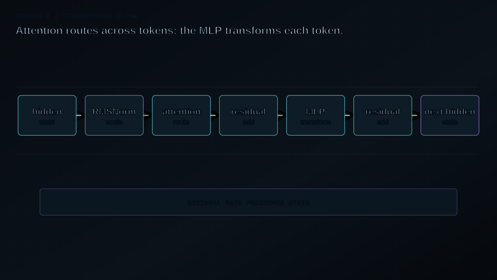

Dense Transformers often use RMSNorm rather than LayerNorm. RMSNorm rescales a vector based on its root mean square value. At the level of intuition, it keeps hidden-state magnitudes in a range that makes deep computation trainable and stable. For inference, the key detail is that it operates per token vector, not across tokens.

That last detail matters for inference. RMSNorm does not mix information between positions. If a prompt has 1,000 tokens, RMSNorm applies the same kind of per-vector rescaling to each token independently. It is part of the per-token path, not the communication path. The same is true of elementwise operations around the MLP.

The MLP also operates per token. A common gated variant is GeGLU:

\mathrm{MLP}(x) = W_2\left(\mathrm{GELU}(W_0x) \odot W_1x\right)

The activation and gate matter for model quality, but the systems-level fact is more direct: the MLP is mostly matrix multiplication. It expands the hidden dimension into a larger intermediate space, applies a nonlinearity and gate, then projects back.

In dense decoder blocks, the MLP is often one of the largest consumers of arithmetic. It has no attention matrix and no notion of which token can see which other token. Its cost comes from width: expanding the hidden dimension and projecting it back turns much of the block's work into wide matrix multiplication.

Attention is where tokens talk to each other.

3. Attention as Information Routing

Self-attention starts by creating queries, keys, and values:

Q = XW_q,\qquad K = XW_k,\qquad V = XW_v

The routing step then scores allowed query-key pairs and mixes values:

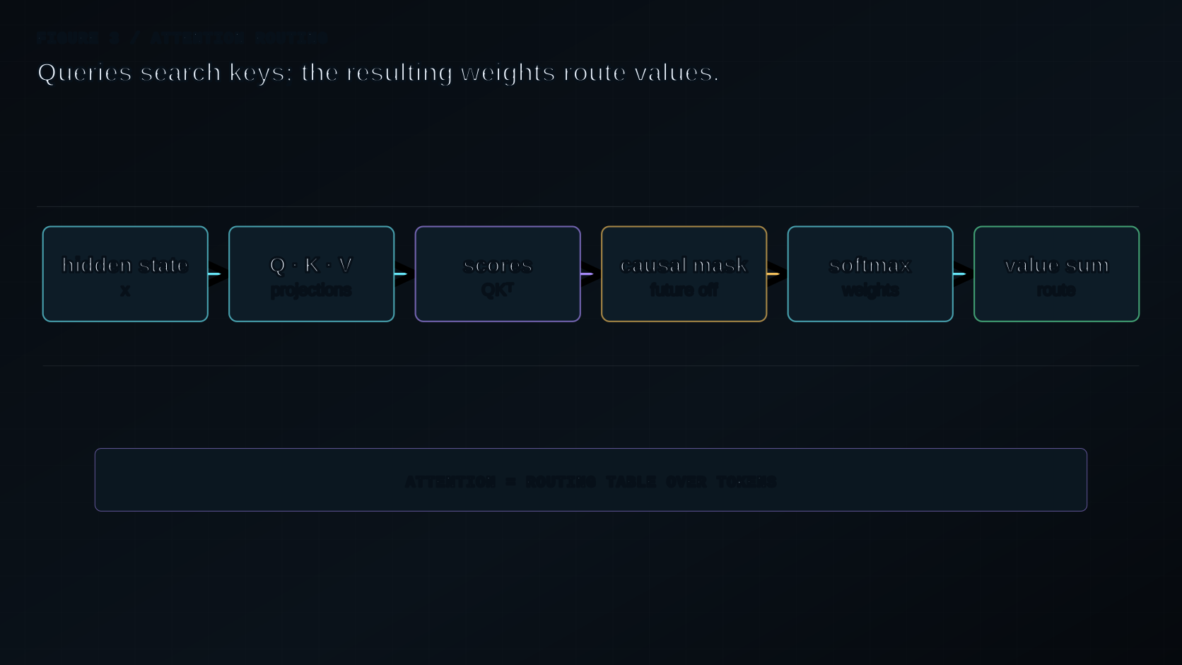
\mathrm{Attention}(Q,K,V) = \mathrm{softmax}\left(\frac{QK^\top + M}{\sqrt{d_k}}\right)V

A diagram of attention routing from hidden states into Q, K, V, mask, softmax, attention weights, and weighted sum. — Figure 3. Attention turns hidden states into queries, keys, and values, applies the causal mask, and uses the resulting weights to route information.

For each token, the query asks what information it is looking for. Keys describe what each token offers as an address. Values hold the information to be mixed into the output. The attention score between one query and one key decides how much that token should read from that value.

The analogy is imperfect, but it captures the inference-relevant part: attention routes information between allowed token positions.

Multi-head attention runs several attention operations in parallel, giving the model multiple routing subspaces. Grouped-query attention reduces the number of key and value heads relative to query heads. That reduces KV-cache size and bandwidth while preserving many query heads. This is one place where architecture already anticipates serving cost.

Grouped-query attention is model design meeting system constraints. The model can keep many query heads, which preserves multiple ways for the current token to ask for information. Key and value heads can be shared across groups of query heads, which reduces the historical state that must be stored and read. The model-level description is "fewer K/V heads than Q heads." The serving-level consequence is fewer cache bytes per token and less bandwidth pressure during decode.

Attention is also where sequence length enters most visibly. During prefill, each token can attend to previous allowed tokens, so the work grows with the prompt. During decode, the new token attends to the cached history. The model only computes the newest query, key, and value, but it still has to read old keys and values. That is why decode often shifts attention from arithmetic to memory access.

The attention output is then projected back into the hidden dimension and added through a residual connection. The token now contains information gathered from earlier allowed positions.

The MLP/attention distinction pays off during inference. If a token needs to rewrite its internal features, the MLP is the obvious place. If it needs to borrow information from the prompt, attention is the path.

4. Masks Define What Tokens Are Allowed to See

Attention does not automatically mean every token can read every other token.

The mask defines the information flow graph. In a causal language model, token i can attend to token j only when j <= i. Future tokens are masked out, because the model is trained and used to predict the next token from the past.

When training data is packed, segmentation masks may also prevent tokens from separate documents from attending into each other. Without that, packing could leak information across unrelated examples.

Segmentation masks are a good reminder that "context" is not simply the tokens that happen to sit nearby in memory. It is the graph allowed by the mask. Two documents can be packed into one sequence for efficiency, but if the mask blocks cross-document attention, their hidden states should not exchange information. The tensor is shared; the information flow is not.

For long-context models, the mask may be more structured. Some layers may use local attention, where a token can only see a recent block of context. Other layers may use global attention, where tokens can attend across the full sequence. This hybrid pattern changes the cost and information path. A token may not reach every earlier position in every layer, but global layers give it periodic long-range access.

The attention mask is the network topology inside the sequence. It decides which hidden states can exchange information; the weights decide how strongly they exchange it.

5. Positional Encoding and Long Context

Attention scores compare queries and keys. Without position, the model would have a hard time distinguishing the same token appearing early or late. Positional encoding injects order into the representation.

RoPE rotates query and key coordinates as a function of position. Because attention later takes dot products between rotated queries and keys, relative position affects the score. YaRN extends this idea to support longer contexts by adjusting the frequency behavior used in the rotations.

Long context is more than a longer input array. It increases attention work, KV-cache memory, and the amount of prefill before the first generated token. It also changes batching: one long prompt can consume far more compute and memory than a batch of short prompts, and it can alter the payoff from prefix caching, chunked prefill, and scheduling policies.

There is also a quality side to the systems choice. A model may support a large context window, but that does not make all tokens equally cheap or equally relevant. Far-away tokens still occupy cache. They still affect attention behavior. They can change latency even if the answer depends on a small part of the prompt. Long context is both a capability and a cost center.

At the model level, long context is a capability. At the serving level, it is a resource problem.

6. From Hidden State to Logits

After the final Transformer block, each position has a hidden state. For next-token prediction, the model usually uses the hidden state at the last generated position. A final projection maps it to vocabulary-sized logits:

\mathrm{logits}_t = h_t W_{\mathrm{vocab}}

If the vocabulary has 128,000 entries, this projection produces 128,000 scores. Sampling logic then chooses a token according to temperature, top-p, top-k, greedy decoding, grammar constraints, or other decoding rules.

The chosen token becomes part of the sequence. During generation, the model repeats the process autoregressively.

This loop is the source of both the power and the cost of LLM inference. The model generates flexible text because each new token is conditioned on the previous sequence. The service pays for that flexibility because each generated token requires another forward pass through the model.

Sampling is the last model-facing step before the serving system sees a new output token. Greedy decoding, temperature, top-p, top-k, and grammar constraints do not change the Transformer block itself, but they change which token is appended and when generation stops. That means decoding policy can affect both output behavior and serving cost. A request that stops after ten tokens releases cache quickly. A request that generates a thousand tokens keeps growing cache and re-enters the scheduler many more times.

7. KV Cache Connects Architecture to Serving

During prefill, the model computes keys and values for all prompt tokens. During decode, newly generated tokens need to attend to previous tokens. The naive approach would recompute keys and values for the whole history every time. That would waste enormous work.

Within a standard causal decode pass, previous keys and values do not change when a new token is appended. They can therefore be computed once and stored. That statement assumes the same model parameters, positional convention, and prefix; editing or replacing earlier context creates a different cache-validity problem.

That stored state is the KV cache.

For a single request, the idea is straightforward:

prompt tokens -> compute K/V -> store cache
new token -> compute new K/V -> append cache
next token -> read old K/V + append new K/V

For a serving system, the idea becomes harder. Each active request owns cache. Longer prompts own more cache. Longer generations keep growing cache. Concurrent users compete for the same GPU memory. Prefix caching can reuse cache when prompts share an initial segment. Paged attention can reduce fragmentation by storing cache in blocks rather than large contiguous chunks.

It helps to separate prefill cache creation from decode cache use.

During prefill, the model processes the prompt and writes keys and values for all prompt positions. This is the expensive setup phase. It creates the memory that later decode steps will use.

During decode, the model writes keys and values for the newly generated token and reads keys and values for the existing history. For an unchanged causal prefix, the old entries remain valid. The cache works because the computation for earlier positions does not need to be revisited when only a new suffix token is appended.

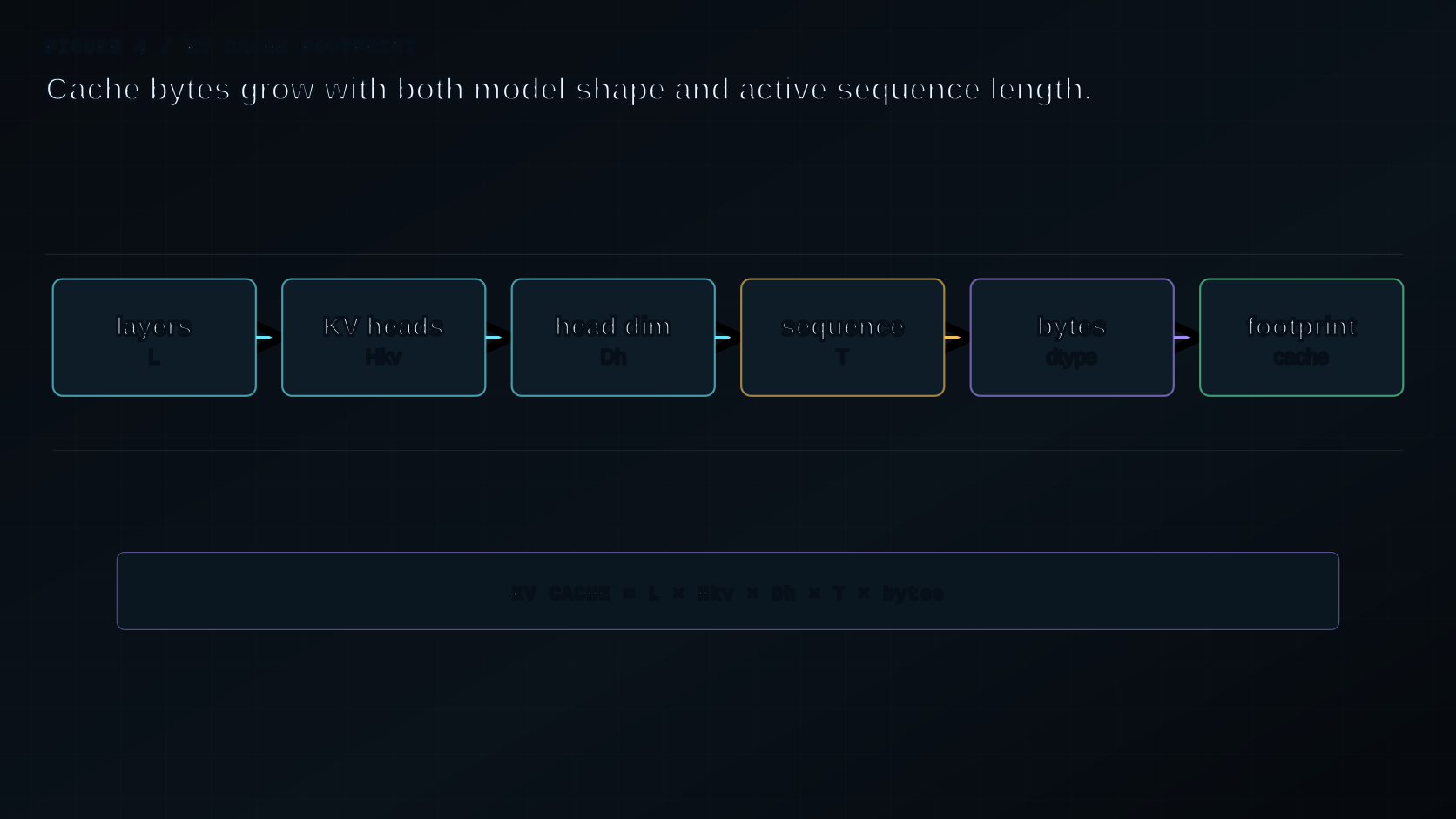
The cache also explains why inference serving does not scale only with parameter count. Two models with similar weight size can behave differently under long-context traffic if their KV-cache footprint differs. Number of layers, number of K/V heads, head dimension, dtype, and active sequence length all affect how many bytes are needed per token. The Transformer architecture has already made a serving commitment before the scheduler sees a single request.

For a rough memory estimate, each cached token stores both keys and values across layers:

\mathrm{KVBytes} \approx 2 \cdot L \cdot H_{\mathrm{kv}} \cdot d_{\mathrm{head}} \cdot S \cdot b

Here $L$ is the number of layers, $H_{\mathrm{kv}}$ is the number of key/value heads, $d_{\mathrm{head}}$ is head dimension, $S$ is active sequence length, and $b$ is bytes per scalar.

A diagram showing KV cache footprint as layers times KV heads times head dimension times sequence length times bytes. — Figure 4. KV-cache footprint grows with layers, key/value heads, head dimension, sequence length, and numeric precision.

At this point, Transformer architecture starts to look like serving architecture. The model says attention needs keys and values from earlier tokens. The serving engine has to decide where those keys and values live, how they are addressed, and which request gets memory next.

That question sits outside the clean Transformer diagram, but the architecture creates it. Once the model reuses old keys and values, the serving system inherits a state-management problem: how many requests can own cache at once, and how expensive is each cached token?

Before getting to the engine side, there is one more layer to examine: the expensive arithmetic behind those projections.

Diagram: Token Flow Inside the Transformer

flowchart TD A["Raw text"] --> B["Token IDs"] B --> C["Embedding vectors"] C --> D["Transformer block 1"] D --> E["Transformer blocks 2 to N"] E --> F["Final hidden state"] F --> G["Vocabulary logits"] G --> H["Sampled next token"] subgraph Block["Inside one Transformer block"] I["RMSNorm"] --> J["Attention: cross-token communication"] J --> K["Residual add"] K --> L["RMSNorm"] L --> M["GeGLU MLP: per-token transformation"] M --> N["Residual add"] end

The Transformer view now leaves a concrete set of systems constraints on the table. Prefill and decode differ because prefill processes a whole prompt while decode adds tokens one step at a time. KV cache exists because autoregressive attention can reuse previous keys and values. Long context increases both computation and memory pressure. The expensive projections inside attention and MLP blocks are mostly matrix multiplications, which means the next diagnosis moves from model structure to GPU shape.

Key Takeaways

A Transformer sees token-indexed vectors, not raw language strings.
MLPs rewrite each token vector; attention lets tokens read from allowed positions.
Masks and positional encodings decide which context a token can use and how expensive that context becomes.
KV cache avoids recomputing old keys and values during decode.
The cache that makes decode practical also becomes a serving-system memory constraint.

Citation

Please cite this article as:

Ji, Wenbo. “The Life of a Token Inside a Transformer”. fusheng-ji.github.io (May 2026). https://fusheng-ji.github.io/blog/posts/life-of-a-token-transformer/

Or use the BibTeX entry:

@article{ji2026lifeofatokentransformer,
  title = {The Life of a Token Inside a Transformer},
  author = {Ji, Wenbo},
  journal = {fusheng-ji.github.io},
  year = {2026},
  month = {May},
  url = {https://fusheng-ji.github.io/blog/posts/life-of-a-token-transformer/}
}

References

Aleksa Gordic, Inside the Transformer: The Life of a Token.
Vaswani et al., Attention Is All You Need.
Zhang and Sennrich, Root Mean Square Layer Normalization.
Shazeer, GLU Variants Improve Transformer.
Su et al., RoFormer: Enhanced Transformer with Rotary Position Embedding.
Peng et al., YaRN: Efficient Context Window Extension of Large Language Models.
Shazeer, Fast Transformer Decoding: One Write-Head is All You Need.
Ainslie et al., GQA: Training Generalized Multi-Query Transformer Models from Multi-Head Checkpoints.

Note: This blog was drafted and polished with assistance from ChatGPT, based on my reading notes on Aleksa Gordic's Transformer, matmul, and vLLM articles. Illustrations were generated with GPT Image 2.

#llm-inference