A Token's Journey Across the LLM Stack
A unified mental model for token computation, GPU execution, memory, and serving.
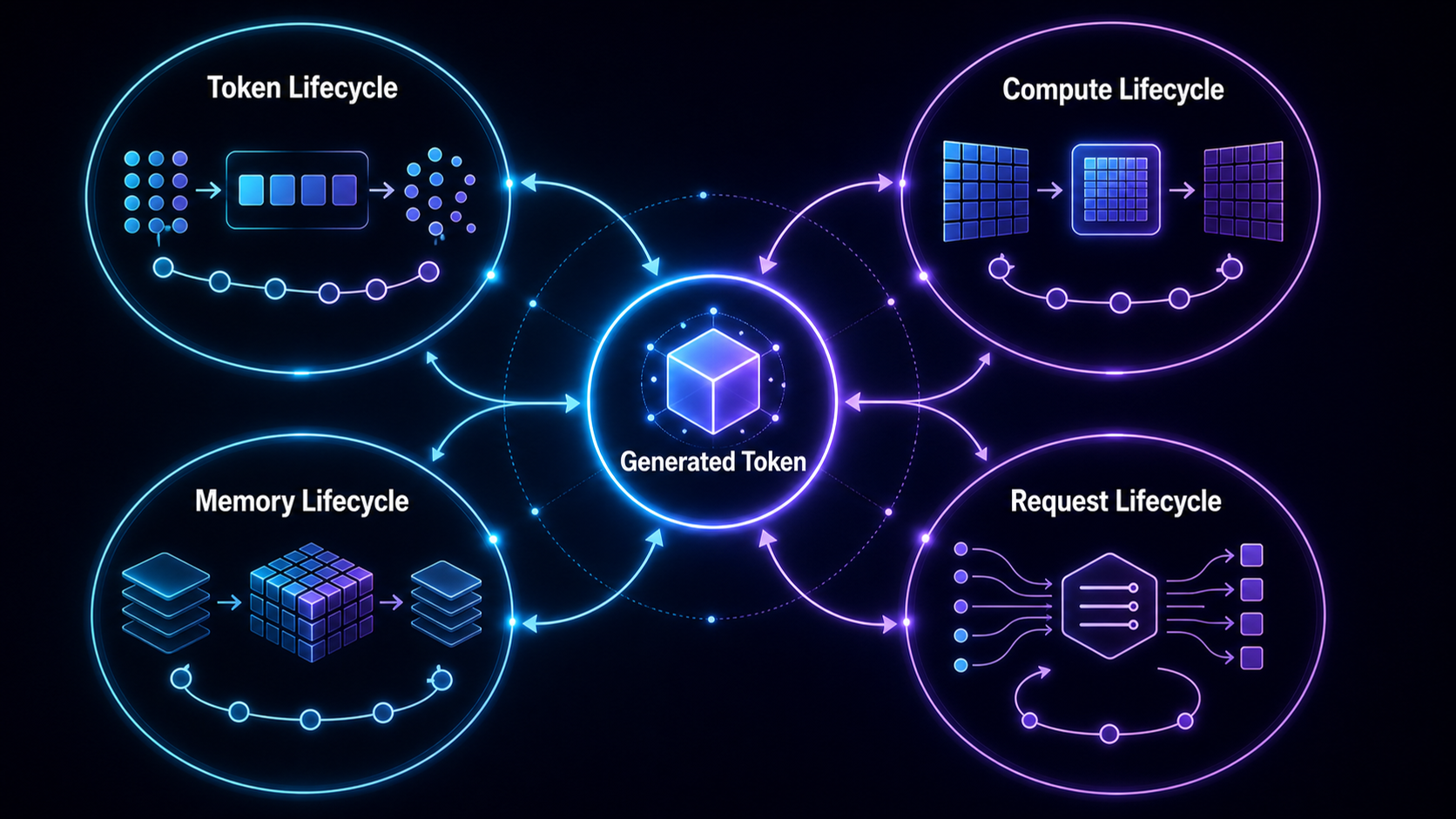
Modern LLM inference is easier to debug when one generated token is separated into four lifecycles: token, compute, memory, and request. The token is represented inside the model, executed by GPU kernels, stored partly in KV cache, and scheduled as part of a live request.
There is no single place where "the next token" happens. A slowdown can come from the model shape, the kernel shape, the cache state, or the scheduler's current batch. Keeping those layers separate makes the first measurement less arbitrary.
This post uses four lifecycles:
- Token lifecycle.
- Compute lifecycle.
- Memory lifecycle.
- Request lifecycle.
Each lifecycle has its own objects and failure modes. Under load, they interact.
The split keeps measurements attached to causes. Token lifecycle questions identify what the model has to compute. Compute lifecycle questions show how that work maps to hardware. Memory lifecycle questions track what state persists across steps. Request lifecycle questions show how many users share the same resources.
The same symptom can involve all four. A long time to first token may come from a long prompt, inefficient prefill kernels, cache allocation pressure, or a scheduler that queues the request behind other work. If those layers are not separated, debugging becomes guesswork.
1. Token Lifecycle
The token lifecycle is the model-level view.
text
-> token ID
-> embedding vector
-> contextual hidden state
-> logits
-> sampled next token
The raw prompt is converted into token IDs. Each ID indexes an embedding vector. The vector passes through Transformer blocks, where attention lets it gather context and MLPs transform its features. The final hidden state is projected into logits over the vocabulary. Sampling logic chooses the next token.
This path explains why masks matter, why position matters, why attention cost grows with context, and why a generated token depends on previous tokens.
It also explains why inference is sequential at the output level. The model cannot know token t + 1 until token t has been chosen, because token t becomes part of the next input context.
The token lifecycle is the right place to ask whether the requested computation is intrinsically expensive. A wider hidden size, more layers, more heads, a larger vocabulary, or a longer context all increase the model-side work before the GPU implementation is even considered. If the architecture asks for more computation per token, no scheduler can make that cost disappear.
At a coarse level, model-side token cost scales with layer count, sequence length, and hidden width:
It also clarifies what "one token" means. A generated token is not a character or a word. It is an index sampled from logits. Before it appears as text, it has passed through embedding lookup, repeated representation updates, attention routing, MLP transformation, final projection, and sampling. That is the model-level path.
2. Compute Lifecycle
The compute lifecycle is the kernel-level view.
linear projection
-> matrix multiplication
-> tiled GPU kernel
-> tensor core execution
The model says "apply this linear layer." The GPU sees a matrix multiplication. The kernel breaks it into tiles, moves those tiles through memory hierarchy, and feeds tensor cores with fragments.
This path explains utilization. A model can have a known FLOP count and still run poorly if the kernels do not use the hardware well. Data may arrive too slowly. Tile shapes may be wrong. Batch sizes may be too small. Attention kernels may be limited by memory bandwidth rather than arithmetic throughput.
The compute lifecycle is where equations become hardware behavior.
The kernel question is whether the work is limited by arithmetic or data movement:
The compute lifecycle is the right place to ask whether the GPU is doing the kind of work it is good at. Large regular matmuls can be efficient. Small irregular decode batches may be less efficient. Attention kernels may shift from compute-heavy to memory-heavy depending on cache reads. Quantization may reduce memory traffic, but only if the kernels and hardware path use it well.
Benchmark results split along the same line. A model may show excellent throughput in a prefill-heavy test and weaker latency in decode-heavy traffic. Both results can be true. They exercise different shapes and different parts of the compute lifecycle.
3. Memory Lifecycle
The memory lifecycle sits between model and serving.
activation
-> Q/K/V tensors
-> KV cache
-> cache blocks
-> prefix reuse
During prefill, activations produce keys and values for every prompt token. During decode, previous keys and values are reused. That cache grows as generation continues.
Inside a serving engine, cache becomes block allocation. Paged attention maps logical token positions to physical cache blocks. Prefix caching can reuse cache for repeated prompt prefixes. Finished requests release blocks back to the pool.
This path explains why VRAM becomes the bottleneck even when there is enough compute. Long contexts, many concurrent requests, and large key/value dimensions can consume memory quickly. Fragmentation and allocation policy can reduce effective capacity. Cache eviction can change latency and recomputation cost.
Memory is not passive storage in LLM serving. It shapes the schedule.
The memory lifecycle asks whether the system is constrained by state. KV cache is the obvious object, but it is not the only one. Weights, activations, temporary workspaces, communication buffers, and allocator behavior all affect how much active work fits on the accelerator. Under long-context or high-concurrency workloads, KV cache often becomes the limiting resource because it grows with active sequence length.
One simple pressure ratio is active cache demand over available cache capacity:
Memory pressure changes behavior before it becomes an out-of-memory error. The scheduler may admit fewer requests. Prefix cache entries may be evicted. Long prompts may be delayed. Cache fragmentation may reduce effective capacity. These effects show up as latency and throughput changes, not merely in memory dashboards.
4. Request Lifecycle
The request lifecycle is the serving-level view.
request arrives
-> prompt is prefilled
-> KV cache is allocated
-> decode steps are scheduled
-> tokens stream back
-> request finishes
-> cache is released
A request enters the system with a prompt and sampling parameters. The engine tokenizes it, schedules prefill, allocates KV cache, then repeatedly schedules decode steps until completion.
This path explains latency and throughput. Time to first token depends heavily on prefill and queueing. Inter-token latency depends on decode scheduling, batch shape, cache reads, and model execution. Tail latency depends on how the scheduler handles long prompts, long generations, and memory pressure.
The request lifecycle is where individual token generation becomes an online service.
The request lifecycle tracks what the user experiences. Time to first token includes queueing and prefill. Inter-token latency includes decode scheduling and model execution. Tail latency includes interactions with long prompts, memory pressure, and bursts. Throughput includes how well the engine keeps the GPU occupied across many changing requests.
Throughput is a serving outcome, not only a model property:
A request is also the unit of policy. The engine can prioritize, delay, admit, reject, preempt, batch, stream, and finish requests. Those choices are invisible in the Transformer equation, but they dominate production behavior.
5. The Four Lifecycles Interact
The lifecycles are separate only for analysis.
A long prompt begins as a token lifecycle issue: more tokens. It becomes a compute issue because prefill has more work. It becomes a memory issue because KV cache is larger. It becomes a serving issue because long prefill can delay other decode requests.
A large hidden size begins as a model architecture choice. It becomes larger matmuls, more memory movement, more KV-cache bytes per token, and higher cost per scheduled step.
A small active decode batch begins as a traffic shape. It becomes poor GPU utilization because kernels do not have enough parallel work. The serving engine may try to batch more requests, but that can increase latency.
Prefix reuse begins as a prompt pattern. It becomes a memory question because cached prefixes occupy VRAM. It becomes a scheduling question because reused prefixes can reduce prefill cost but require cache lookup and lifecycle management.
Single-layer explanations often fail. "The GPU is slow" may really mean the scheduler is feeding it poor shapes. "The model is too large" may really mean KV cache is limiting concurrency. "Decode is slow" may mean memory bandwidth is the bottleneck, not tensor-core arithmetic.
The interactions are also why local optimizations can disappoint.
A faster matmul kernel helps only if matmul is the bottleneck for the active workload. More VRAM helps only if the scheduler and cache manager can use the extra capacity. Prefix caching helps only if prompts repeat and cache entries survive long enough to be reused. Speculative decoding helps only if draft tokens are accepted often enough to offset the extra work.
The full-stack view does not make optimization easier. It makes wrong optimizations easier to spot.
Unified Diagram
The diagram loops because inference loops. A generated token changes the token sequence, extends memory, triggers more compute, and updates request state.
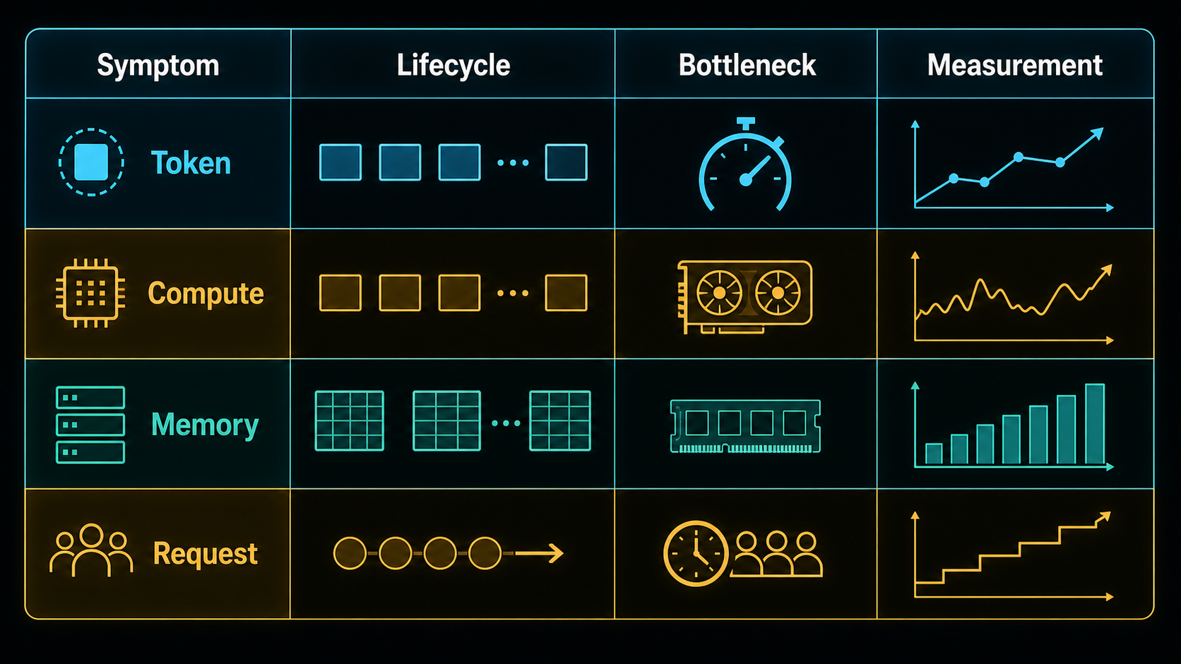
6. Diagnostic Framework
When an LLM system is slow, separate the symptom into four questions.
Model Question
Is the architecture expensive?
Examples:
- Large hidden size.
- Many layers.
- Many attention heads.
- Long context.
- Large vocabulary projection.
A model with more layers or wider hidden states increases work per token. More heads and larger key/value dimensions increase attention and cache cost. Long context increases prefill work and cache memory. A large vocabulary projection can become noticeable, especially for small decode batches.
The model question checks whether the requested computation is heavy before blaming implementation.
Kernel Question
Are GPU kernels efficient?
Examples:
- Poor matmul utilization.
- Memory bandwidth bottleneck.
- Low tensor core occupancy.
- Inefficient attention kernels.
Kernel issues show up when theoretical throughput is high but delivered performance is low. The GPU may be underfed because batches are too small. Kernels may spend too much time moving data. Attention may be dominated by KV-cache reads. Quantization may help memory bandwidth but only if the kernels are good.
The kernel question checks whether the computation is mapped well to the hardware.
Memory Question
Is KV cache the bottleneck?
Examples:
- Long context.
- Many concurrent users.
- Fragmentation.
- Cache eviction.
- Insufficient VRAM.
KV cache can quietly become the limiting resource. A service may have compute capacity left but no memory for more active requests. Cache block size, paging policy, prefix reuse, and eviction behavior all affect effective throughput.
The memory question checks whether the system is limited by state, not arithmetic.
Serving Question
Is scheduling inefficient?
Examples:
- Poor batching.
- Long prefill blocking decode.
- High tail latency.
- Low concurrency.
- Prefix reuse not exploited.
A scheduler can make a good model and good kernels look bad. If it admits too much prefill at once, decode latency suffers. If it batches too conservatively, GPU utilization falls. If it ignores repeated prefixes, it recomputes avoidable work. If it pushes concurrency too high, memory pressure creates instability.
The serving question checks whether the engine is organizing work around real traffic well.
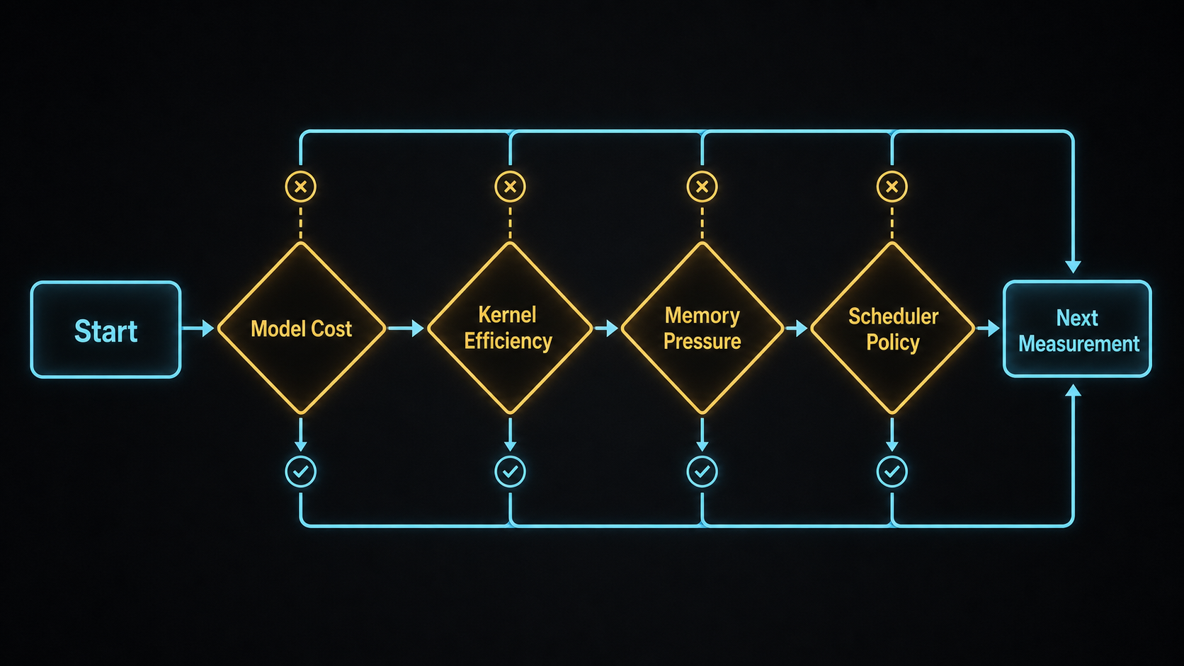
How to Use the Framework
Start with symptoms, then choose the first layer to measure.
High time to first token points first to prompt length, queueing delay, prefill chunking, and prefix cache hits.
High inter-token latency points first to decode batch size, KV-cache bandwidth, attention kernels, and scheduler policy.
Low throughput with acceptable latency points first to GPU utilization and batch formation.
Latency spikes under load point first to cache pressure, request length distribution, prefill/decode prioritization, and tail behavior.
If adding GPUs does not help, inspect parallelism strategy and communication overhead. Tensor parallelism can fit larger models, but it adds communication. Pipeline parallelism can introduce bubbles. Data parallelism helps throughput only if routing and load balancing are effective.
The checklist helps only if it prevents measuring the wrong layer first.
Here is a compact symptom map:
| Symptom | First lifecycle to inspect | Common causes |
|---|---|---|
| High time to first token | Request + compute | queueing, long prefill, poor prefill batching, missed prefix reuse |
| High inter-token latency | Memory + request | KV-cache bandwidth, small decode batches, scheduler policy |
| Low GPU utilization | Compute + request | inefficient batch shapes, too little active work, launch overhead |
| VRAM fills quickly | Memory | long contexts, many active requests, large K/V dimensions, fragmentation |
| Good benchmark, poor product latency | Request | benchmark traffic does not match online arrival and output patterns |
| More GPUs do not help | Compute + request | communication overhead, poor routing, imbalance, pipeline bubbles |
The table is not complete, but it enforces the sequence: name the symptom, name the lifecycle, then choose the measurement.
The next split is capacity versus policy. Capacity asks what the hardware and model can support: memory, bandwidth, compute, and cache blocks. Policy asks how those resources are assigned: which request enters, which prefill is chunked, which cache entry is retained, and which batch shape is formed. Many production failures are policy failures under capacity pressure.
Buying more hardware can increase capacity, but it does not automatically fix bad batching, missed prefix reuse, or unfair scheduling. A better scheduler can improve policy, but it cannot make an architecture with a huge KV-cache footprint cheap under long-context traffic. The lifecycles help identify which kind of fix is actually being proposed.
The same distinction applies to model changes. A smaller model changes capacity pressure by reducing compute and memory cost. A longer context window changes demand by letting requests bring more tokens. A new decoding method changes policy by altering how work is scheduled and verified. Treating all of these as "inference optimization" hides the mechanism. The lifecycle view keeps the mechanism visible.
The aim is not to make every engineer an expert in every layer. It is to make a diagnosis specific enough to name the object, the lifecycle, the bottleneck, and the measurement that would prove it. Without that, every symptom turns into a generic speed problem. With it, the next experiment is usually clearer.
Conclusion
A token begins as an integer and ends as another integer sampled from logits. The object is small, but the path between those integers crosses the entire LLM stack.
The Transformer gives the token a contextual representation. GPU kernels execute the expensive matmuls and attention operations. Memory systems store activations and KV cache. Serving systems schedule requests, batch work, reuse prefixes, and release cache when the request ends.
Use this as a debugging vocabulary rather than only as a diagram. Instead of asking whether "the model is slow," ask whether the bottleneck is architecture, kernel execution, memory state, or serving policy. Those questions lead to different measurements and different fixes.
It also keeps optimizations honest. A faster kernel may not help if decode is dominated by KV-cache bandwidth. A better scheduler may not help if the model is too large for the latency target. More memory may increase concurrency, but only if batching and admission control can use it. The next-token interface is simple; the system behind it is constrained by shapes, cache, and policy.
Key Takeaways
- A generated token has four lifecycles worth separating: token, compute, memory, and request.
- Token lifecycle explains hidden states and logits; compute lifecycle explains tiled GPU work.
- Memory lifecycle explains KV-cache pressure; request lifecycle explains scheduling and latency.
- The same symptom can come from model shape, kernel efficiency, cache state, or serving policy.
- Inference debugging should name the lifecycle, bottleneck, and measurement before choosing a fix.
Series Navigation
- Part 0: LLM Inference Is a Full-Stack Systems Problem
- Part 1: The Life of a Token Inside a Transformer
- Part 2: Why Transformer Performance Is Mostly a Matmul Problem
- Part 3: The Life of a Request Inside vLLM
- Part 4: A Token's Journey Across the LLM Stack (current)
References
- Aleksa Gordic, Inside the Transformer: The Life of a Token.
- Aleksa Gordic, Inside NVIDIA GPUs: Anatomy of high performance matmul kernels.
- Aleksa Gordic, Inside vLLM: Anatomy of a High-Throughput LLM Inference System.
- vLLM Project, vLLM Documentation.
Note: This blog was drafted and polished with the assistance of ChatGPT (GPT-5.4 Thinking), based on my reading notes on Aleksa Gordic's Transformer, matmul, and vLLM articles. Illustrations were generated with GPT Image 2.
- ← Previous
The Life of a Request Inside vLLM - Next →
Embodied AI World Models